How Concatenate in Excel Works
The Concatenate function is straightforward to use. The syntax for the function works as follows: CONCATENATE(text1, text2, text3, …) This function appears very simple. It will string together multiple text strings into a single string. You place each string (or the cell that holds the string) separated by commas inside the function.
While it may be simple, its uses are plentiful. In this article, we’ll go over a few examples of some of the most useful ways you can use the Concatenate function in your various projects.
1. Formatting Names
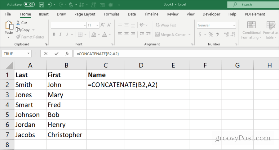
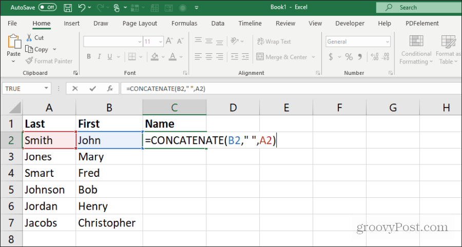
One of the most common uses for the Concatenate function is when your spreadsheet contains names in two columns, like in the example above. This is one of the easiest ways to use this function since it involves stringing together two columns with a space in the middle. The syntax for this is: CONCATENATE(B2,” “, A2)
This will put the first name and the last name in the correct order, with a space in the middle. To fill the rest of the column for the other names, hold down the Shift key on the keyboard and double click.
This will autofill the column with the rest of the names.
2. Update a Status in Plain Language
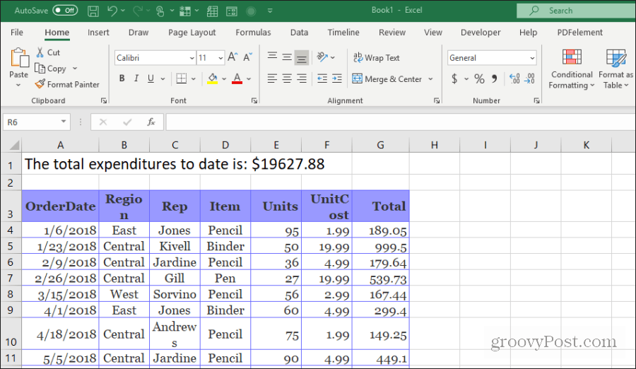
You may use a spreadsheet to put together a large amount of data to perform a complex series of calculations whenever you open the sheet. But all you really care about is the end calculation. Save time by using Concatenate to craft a status with the final result at the very top of the sheet. If the calculated result is in cell G47, you will use the following formula to create an updated status in cell A1: =CONCATENATE(“The total expenditures to date is: $”, G47) This will result in the statement at the top of the spreadsheet, as shown below.
Now you can save some time by just opening the sheet and getting the result at a glance.
3. Parse a Mailing Address
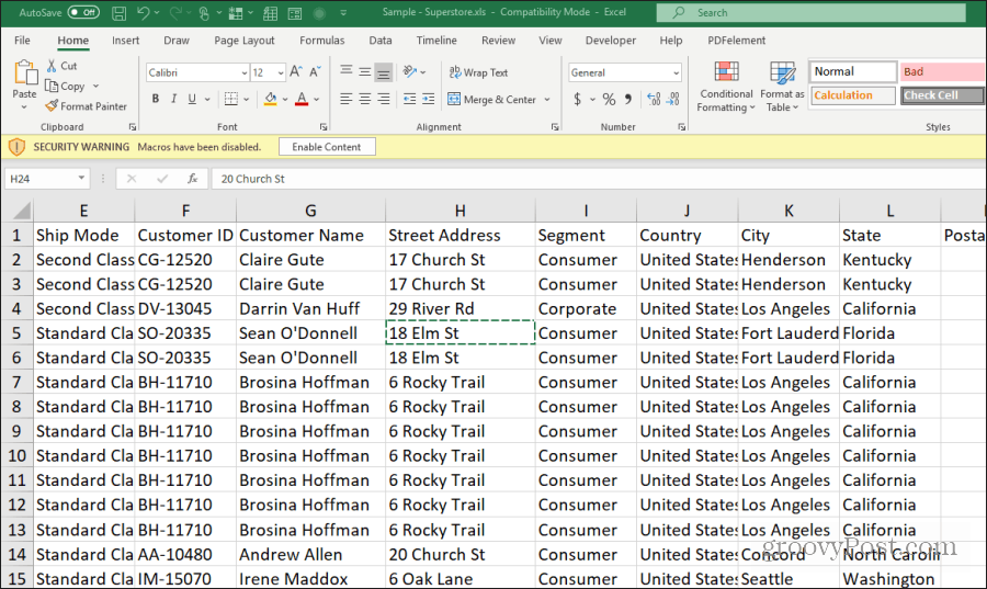
One of the most popular uses for the Concatenate function is taking various fields in a database filled with information from users, customers, or anyone else and piecing together their full address into a single field. This way, you can grab the entire address with a quick right-click and copy. Your spreadsheet may have pieces of the address split up among fields spread across the entire table.
You can build a formatted address by stringing the pieces of the address into one cell, separated by a carriage return. In Excel, that’s “Char(10)”. You’d piece together the address using the following function: =CONCATENATE(G2,CHAR(10),H2,CHAR(10),K2,”,”,L2,” “,M2) The carriage return code goes after the name and the street, and the city, street, and zip code need to be formatted with a comma and a space. The result may actually look like a jumbled mess. This is because you need to format the address cells with Wrap text. Do this by selecting all of the address cells, right-clicking, and selecting Format Cells. In the Format Cells window, select the Alignment tab and enable Wrap text.
Now you’ll see that all of the addresses are formatted as expected.
This approach can be used for any field where you want to create formatted text that pulls together data from throughout the spreadsheet.
4. Parse Together a URL
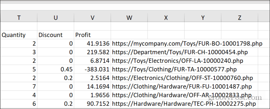
Another good use for the Concatenate function is piecing together all of the elements for a full URL string. For example, the URL link to the purchased product may be made up of the site domain, the department, and the Product ID in the product spreadsheet.
For each row, you can build the URL using both static and dynamic addressing for cells. =CONCATENATE(“https://”,D1,”/”,D3,”/”,O3,”.php”) This attaches the static text “HTTPS:” to the beginning and “.php” to the end of the URL string for that product. You’ll insert the URL segments by selecting the cells for the domain, the department, and the product ID between each of the forward slashes. All of these are separated by commas. The result is a perfectly formatted URL link to that product.
You can fill the rest of the cells using the same approach as above. Hold down the shift key and place the mouse at the lower right corner of the first cell where you’ve built the concatenated URL until you see double parallel lines. Double click to fill the rest of the cells in that column with the same function. Cells will automatically adjust for each row.
5. Dynamic Title Charts
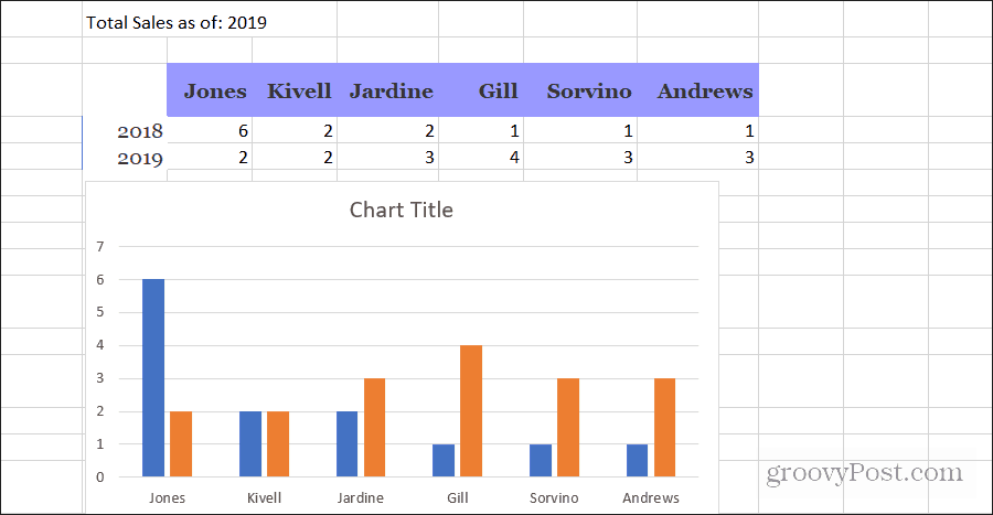
One of the favorite uses of the Concatenate function is to dynamically title charts in a spreadsheet. This is often needed to update things like the current date for a spreadsheet that’s used as a recurring report. For example, in the sales spreadsheet, you can create a title cell that holds the title for the chart. Using the Concatenate function, you can update the current date when you update the spreadsheet. =CONCATENATE(“Total Sales as of: “,YEAR(NOW())) This cell will update with the correct date every time the chart updates.
Next, you have to set the chart title to update with those cell contents. To do this:
Now, whenever the spreadsheet updates, the chart will have the correct date in the title. You don’t have to worry about remembering to update it whenever you run the report.
6. Combine Numbers and Text
Another useful feature of the Concatenate function is that it lets you combine text cells and number cells into one string. You can also bring in dates if you convert the date field to text. For example, to convert each sale event into a plain English statement, you might use a Concatenation function like shown below. =CONCATENATE(C4,” sold “,E4,” units of “,D4,” on “,TEXT(A4,”mm/dd/yyyy”)) This will take two text fields (sales rep name and unit name) and combine them with a number and date field (unit number and date of sale).
This allows you to build an entire text field that you can then use to send out email content from the Excel sheet automatically.
7. Automatically Build HTML
If you take that ability to combine text, values, and other data from your spreadsheet into a single cell of content, and then combine that with the use of the Char(10) newline function and HTML codes, you could build HTML code that you could insert into any web page. A use for this might be copying spreadsheet calculation results into a web page where you provide the calculation results to the public (or to your internal corporate network). For example, let’s say that you’re running a book club website and post weekly updates to members with the latest reading material for the month. If you use a spreadsheet to log each monthly update, you can use Concatenate to build the page content for that entry.
Create another cell for the web page content, and then Concatenate your content using cell entries from the sheet: =CONCATENATE(“Hello again everyone!
”,CHAR(10), “This month we’re going to be reading ”,A2,” by ”,B2,”.
”,Char(10),” This title was published in ”,C2,”.”, ” I’m looking forward to hearing what you all think!”) As you can see, combining static strings, information from cells, and formatting codes combined with HTML formatting codes lets you create any content at all that dynamically pulls information from your spreadsheet.
With a little creativity, you could generate a lot of page content. And copy and paste it directly into your blog posts.
8. Generate Codes
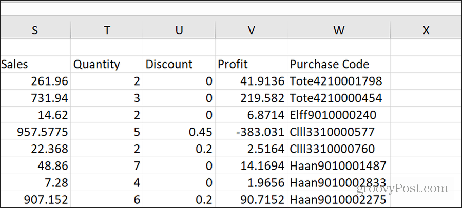
Another useful trick you can use concatenate is to piece together sections of information from each field into a special code. You can use that code as a unique identifier. Using the product spreadsheet example, let’s say you want to create a unique code to identify every individual purchase made on the website. In this example, the purchase code will be made up of:
The first two letters of the departmentThe last two letters of the customer nameThe first two numbers of the zip codeThe last 8 numbers of the product ID
You can do this all by combining the Concatenate function with Left and Right string functions: =CONCATENATE(LEFT(D3,2),RIGHT(H3,2),LEFT(M3,2),RIGHT(O3,8)) This nests the Left function (grabbing characters from the left) and the Right function (taking characters from the right) into the Concatenate function.
This is useful for creating unique passwords to build a unique website URL slug for web pages.
![]()

